A novel machine learning approach to predict short-term energy load for future low-temperature district heating

Abstract: In this work, we develop machine learning methods to forecast the day-ahead heating energy demand of district heating (DH) end-users in hourly resolution, using existing metering data for DH end-users and weather data. The focus of the study is a detailed analysis of the accuracy levels of short-term load prediction methods. In particular, accuracy levels are quantified for Artificial Neural Network (ANN) models with variations in the input parameters. The importance of historical data is investigated – in particular the importance of including historical hourly heating loads as input to the forecasting model. Additionally, the impact of different lengths of the historical input data is studied. Our methods are evaluated and validated using metering data from a live use-case in a Scandinavian environment, collected from 20 DH-supplied nursing homes through the years of 2016 to 2019. This study demonstrates that, although there is a strong linear relationship between outdoor temperature and heating load, it is still important to include historical heating loads as an input for prediction of future heating loads. Furthermore, the results show that it is important to include historical data from at least the preceding 24 hours, but suggest diminishing returns of including data much further back than that. The resulting models demonstrate the practical feasibility of such prediction models in a live use-case.

Keywords: Low-temperature district heating, short-term load prediction, machine learning, Scandinavian climate.

Introduction

District heating (DH) plays a vital role for the operation of building energy supply systems, which accounted for 35% of global final energy use and 38% of energy-related CO₂ emissions [1]. However, existing DH networks in many cold climates still use rather high supply temperatures, such as 75°C or above [2]. In the face of green energy initiatives, increasing shares of low-energy buildings, and case examples in mild climates, there is a pressing need to transform the existing DH networks toward low-temperature DH (LTDH).

Digitalization and the overall transition towards smart energy systems and cities are placing higher requirements on integration, communication, and cooperation with end-users (buildings) connected to such LTDH networks. As a result, future generations (4th and 5th) of LTDH networks will feature low operating temperatures, and greater integration with the end-users (buildings) and building-sized renewables. However, how to operate such integrations still rely fundamentally on a thorough understandings of heating loads.

Digital solutions for measuring and controlling the network will allow for higher degrees of system optimization with intermittent renewables and heat pumps. This means that short-term predictions of heating loads are essential. But updating all the legacy monitoring facilities is a very costly and lengthy process. There is still a pressing need for more knowledge about what tools are available, and how well these methods can be utilized for load predictions in LTDH applications. At the same time, there is still room for improvement and solutions that can work on top of the existing DH systems, using existing metering data, during this transition period.

 In the studies investigating DH load predictions, a great amount of methods are based on linear regression models, due to the strong linear relationships of heating load with respect to outdoor temperature. These existing methods commonly have not taken full advantage of using data-driven approaches, such as emerging machine learning (ML) models to perform such predictions. Even within those limited publications in the respective areas, it is still not clear what are the key advantages of using such ML approaches, and to what extent the accuracy levels can be quantified, given limited dataset inputs. This study provides a practice of the above raised challenges.

In this work, ML methods was developed to forecast the day-ahead heating energy demand of DH end-users in hourly resolution, by using existing metering data for DH end-users and weather data. The importance of historical data was investigated – in particular the importance of including historical hourly heating loads as input to the forecasting model. Additionally, the impact of different lengths of the historical input data was studied. The feasibility of such models, and their accuracy, are evaluated using data from a live use-case in Scandinavian environment. A detailed analysis of the accuracy levels of short-term load prediction methods are in focus.

Methodology

The study applies combinations of a two-step approach:

Step 1. A thorough understanding of the DH network and building load on annual basis, namely load profiles. This provides an overall view and boundary conditions of DH networks.

Step 2. Based on the definitions of DH load profile, day-ahead prediction models are developed. The model is rooted as an Artificial Neural Network (ANN) model, varying the input parameters, and trained and evaluated using the DH dataset.

To measure and evaluate the performance of the models, the mean squared error (MSE), and the mean absolute error (MAE), were both recorded for each model after training had been completed, using the 2019 test data (that had not been seen by the models during training).

Data inventory

The heating load was measured and collected for 20 separate nursing homes in Scandinavian climate, all located in the city of Trondheim, Norway. All of these buildings are connected to the same DH network, and the measurements were obtained directly from the measuring equipment of the network operator. The data contains the hourly heating loads for each of the buildings, spanning the entire time period from January 1, 2016, to December 31, 2019, obtained from the energy monitoring platform of Trondheim Municipality [9].

For the model construction and evaluation, the average heating load per square meter (W/m²) was calculated across the 20 buildings for each hour. The data were supplemented with hourly outdoor temperature measurements obtained from the Norwegian meteorological station [10] in Trondheim, for the corresponding period.

Load profile development

The load profile was identified using an energy signature (ES) curve in the study. This method has been widely employed for planning and sizing purposes. An ES curve consists of a temperature dependent part, and a temperature independent part, which are divided by changing point temperature (CPT) or heating effective temperature, defined as:

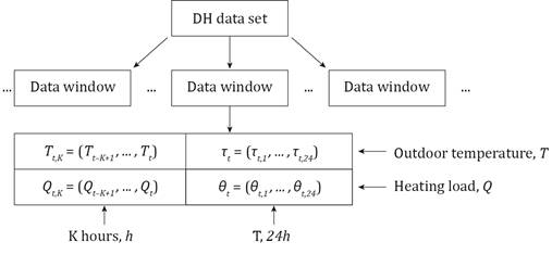
Figure 1. The logic of short-term prediction model.

where Tt is the outdoor temperature at time t, p1 and p2 are the coefficients of each ES curve model, and ε is the residual error. The heating demand follows the linear growth under the slope of p1. Below the changing point temperature, it is the outdoor temperature dependent part and above the changing point temperature, it is the outdoor temperature independent part, when most of the heating needs go to domestic hot water (DHW) use.

For DH network monitoring, the load data are commonly aggregated as a combination of space heating and domestic hot water usage. Therefore, in the energy signature analysis, DHW load is extrapolated based on the existing studies [11], which has reported as a representative DHW profile for the given climate and resident types.

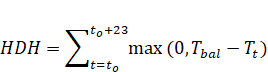
For modelling boundary conditions, daily heating degree hours (HDH) is calculated as the daily summation of the difference between balance temperature and hourly outdoor temperature, see below:

where to is the first hour of the day, the heating balance temperature tbal is assumed at 15°C and negative summands are set to zero. From this, high-heating season, mild-heating seasons and non-heating seasons can be identified in the ES curve.

The day-ahead prediction models

In this study, short-term prediction is defined as 24-hours (day-ahead) time horizon. ANN-based models were developed to predict the short-term heating load, starting from a given hour, for each hour of the following 24-hour period. As mentioned, this serves as a decision-supporting tool for the operation purposes in future LTDH transitions. All of these models used as input the forecasted outdoor temperature for the corresponding 24-hour period. To study the importance of historical data, and the performance impact of different measuring scenarios, nine differentiated ANN models were created and compared.

The models differed in what additional input data were used. One of them used no additional inputs, i.e., only the forecasted outdoor temperature. The other eight models were split into two main categories:

·         Half of them were additionally supplied with the historical outdoor temperature,

·         The other half were supplied, in addition to that, with the historical measured heating load.

For both cases, the historical data were given in the same hourly resolution. Within each category, the models were further differentiated based on the number of hours of historical data stretched back: 12, 24, 48, or 72 hours.

These models had one input layer (the number of inputs varied between the models), one hidden Rectified Linear Unit (ReLU) layer with 64 nodes (this number was determined through hyperparameter search), and one output layer. All the layers were densely connected. Mean squared error (MSE) was used as the loss function, and Adam was used for the parameter optimization, with the maximum number of epochs set to 100.

Mathematical description of the models

The logic of the developed model is presented in Figure 1. Let Qt and Tt represent the measured heating load, and the measured outdoor temperature, at hour t, respectively; and let θt,s and τt,s represent the predicted heating load, and the forecasted outdoor temperature, made at hour t for hour t + s (defined for s = 1,…,24), respectively. Let K be a parameter representing the number of hours of historical measured data to be used as input for the model. Introduce the shorthand notation as,

θt, Qt,K, τt, and Tt,K represent, at the time instance t, the predicted heating load for the following 24 hours, the historical heating load for the preceding K hours (including t), the forecasted outdoor temperature for the following 24 hours, and the historical outdoor temperature for the preceding T hours (including t), respectively.

Each ANN model can then be expressed as either the function

if historical heating load is not an input to the model, or as

if historical heating load is supplied, where fK and gK are abstract representations of our ANN models, and the parameter K takes either of the values 0, 12, 24, 48, and 72 (hours).

Training and evaluation of the models

As mentioned above, the different models were trained and evaluated using the same dataset, introduced in Section “Data inventory”. The dataset was created from the original data by first considering every possible consecutive 24-hour window of both the outdoor temperature and the heating loads, and then appending the preceding K-hour window to it, both for the outdoor temperature and the heating loads. In the cases that did not consider the historical heating load, that part of the window was simply discarded. Each window is therefore split into input and output, according to Figure 1.

The data for the years 2016 and 2017 was used as the training set for the ANN, while the data for 2018 was used as the validation dataset, for the stopping criterion of the training. The resulting models were evaluated using the data for the entire year of 2019, the testing set, to ensure that the models were evaluated on a whole year of data.

Note that the model was evaluated using the actual measured outdoor temperature as the outdoor temperature forecast input. To improve statistical reliability, each model was trained from scratch ten times (using the same training data, but randomly initializing the weights each time), and the averages of these performance measures across the ten iterations were recorded.

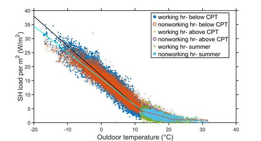
Figure 2. Energy signature (ES) curve for the district heating (DH) load profile.

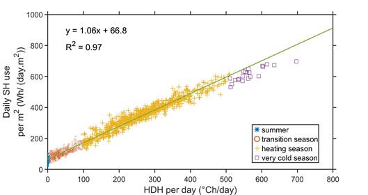
Figure 3. Load characteristics given the whole heating season, presented by heating degree hours (HDH).

Results

ES and load profile characteristics

Figure 2 shows the ES of the DH network. Around 12°C was found as the changing point temperature for providing a proper piece-wise approximation. It is found that outdoor temperature that are above the changing point temperature consists of 22.4% of heating seasons. Figure 2 also shows that space heating loads are less temperature dependent at the mild-heating season (constant slope), and these small loads can be described by one regression line regardless of working hours and non-working hours. The rest 77.6% of the time the outdoor temperature was below the changing point temperature, falls into high-heating season. Along the regression lines below the changing point temperature, there is a small region where non-working hour may need slightly higher space heating load than working hour under the same outdoor temperature (c.a. 10 – 12°C).

From the linear relationship between specific daily space heating and heating degree hours, as displayed in Figure 3, it shows the daily space heating operation follows the daily heating degree hours, without influences from day types or manual false operation/intervention. These results are expected, given the rather high-temperature/conventional DH networks in the study. This also provides the boundary conditions that the day-ahead predictions will be constrained by the operation scenarios, instead of allowing the network temperature drift freely with load variations.

Accuracy levels of day-ahead prediction

The evaluation errors of the models are shown in Table 1. Recall that the evaluation of the models was performed on the dataset covering the entire year of 2019, and that this data had not been previously seen by the model (during the training stage). The results show a clear difference between the models gK that use the historical load data, and the models fK that do not. In particular, the impact of including historical outdoor temperature data, but not historical load, as input to the model is relatively small, even when longer periods of historical temperature data are used, compared to also including the historical load data.

Table 1. Performance measures for the models, evaluated on the testing set of 2019.

Discussion

A significant difference can be observed between the models that use both historical heating loads and outdoor temperature as inputs, and the models that only use historical outdoor temperature. This difference is especially significant during the mild-heating season, when the heating load is dominated by domestic hot water. This is likely due to the relatively weak relationship between outdoor temperature and the total heating load during that period, compared to the high-heating season, when space heating demand is the dominant component. Another reason could be due to thermal inertia and storage effects of the buildings, as well as suboptimal control of the heating loads, in which case the historical heating loads could be useful to model.

This evidence provides a basis for how future LTDH should be operated under different climate conditions, when heating loads fall more into the mild-heating season regime, with perhaps only peaks fall into the high-heating season regime. These differences are also evident in Table 1, which shows the average performance over the whole-year period. The results demonstrate the importance of making historical heating load available to heating load prediction models. Yet, while historical hourly outdoor temperature is often publicly available, historical heating loads are in many cases only available with large delays or low temporal resolution, if at all. The results additionally demonstrate the importance of using historical data from longer time periods, although they seem to suggest diminishing returns beyond the data for the previous 24 hours. This optimal cut-off period will likely differ between different building types, due to differences in thermal inertia.

It should be noted that the performance of the models was evaluated using the actual measured outdoor temperature as the forecasted outdoor temperature for the following 24-hour prediction. In practical applications, this forecast would typically be inaccurate. Such inaccuracies would lead to lower performance than observed in this study. As such, it is important that the base model is as accurate as possible, to reduce the propagation of such inaccuracies within the model.

Conclusions

This study demonstrates that, although there is a strong linear relationship between outdoor temperature and heating load, it is still important to include historical heating loads as an input for prediction of future heating loads. Accuracy levels are quantified by using ANN models with input parameter variations. Furthermore, the results show that it is important to include historical data from at least the preceding 24 hours, but suggest diminishing returns of including data much further back than that. The models developed in this study were evaluated on actual measured data from a live use-case, demonstrating the practical feasibility of such prediction models.

Acknowledgement

This work was financially supported by the Swedish Energy Agency with project No. 51544-1 and EU H2020 programme under Grant Agreement No. 101036656. Special thanks to Trondheim municipality, Norway, for providing data and user information.

References

Please find the full list of references in the original article at: https://proceedings.open.tudelft.nl/clima2022/article/view/319