Heat pumps: lost in standards… and found

Keywords: EPBD – CEN – standards – heat pump

Summary

The draft of the revised EN 15316-4-2 will be published for public enquiry in the next months. This article analyses the main features of this new text.

The calculation procedure has been organised according to a new frame which is independent of the heat pump typology and calculation paths and options. Then the specific features of the two main calculation paths are presented.

“Path A” still requires some discussion and attention on the correction of COP for part load. Several such correction methods are included in the draft to allow testing them. Even the definition of “part load” itself deserves some more attention.

Some more insight is provided about “path B”. The test conditions used in EN 14825 are presented. This makes clear why it’s not straightforward to extract the information on the dependency of the COP from each parameter: they all vary from one test point to the other.

The temperature pattern within the heat pump is illustrated in details, including what happens if the fans of the evaporator and condenser modulate or they do not. This results in a possible trade-off between comfort and energy performance that might be taken into account in the calculation method.

Finally, it is suggested to introduce a mechanism to allow some tolerance for a transient power output deficit of the heat pump when a peak for domestic hot water production occurs. Without this feature, the risk is to invalidate the whole calculation process without a real reason.

Introduction

The former article already introduced EN 15316-4-2 and some basic features of the draft new revision, that should be published for public enquiry in the coming months (late autumn 2021).

This article will analyse more in details the contents and technical background of this new draft.

The frame

There are several types of heat pumps and several possible alternatives for the calculation of the energy performance of heat pumps.

The first concern when drafting this revision was establishing a clear common frame that could:

·         support all the various calculation options for each heat pump typology;

·         guarantee in all cases the connection with the general calculation frame set-up by EN 15316-1;

·         handle several operating conditions in the same calculation interval.

The result is a reviewed step-by-step procedure which is summarised in Annex C of the new draft. For each step, the available alternatives and the reference to the relevant clause are given in tables.

Step 1 is the acquisition of the required energy output per each service provided in the calculation interval. This information comes from the general part EN 15316-1. Currently, the draft supports two services: space heating and domestic hot water. Additional foreseen services can be a direct connection to a hot water storage and space cooling. In fact, now that the frame is defined and working, one realises that it could be used for cooling as well.

Step 2 is the calculation of the source temperature, depending on source type and operating conditions. This is a missing part in the current EN 15316-4-2, which considers only external air. Actually, the issue is only partially solved in the draft revision because there are only simplified models for such sources as ground heat exchangers.

It would be interesting to develop models for the ground exchangers that are also used for free cooling or free heating. Some attention will be required to avoid iterations if the model should take into account the power required from the source: simplifying assumptions like an estimated COP may be a good solution. Sources like ground water and surface water need measured local data.

Step 3 is the calculation of the sink temperature per each service. This is an important information that comes from the general part EN 15316-1. For a correct calculation of heat pump performance, the use of the procedures given in annex C (heating circuit operating temperatures) and D (generators circuit temperatures) of EN 15316-1 is essential. These annexes are basic methods but additional options and related procedures may be developed nationally. An example of a useful additional feature is a simple heating curve (flow temperature as a function of outdoor temperature). Methods in annex C of EN 15316-1 are all based on heat demand, since they were primarily developed for use with a monthly method.

If cooling would be integrated in the frame as an additional service, then the role of source and sink in steps 2 and 3 shall be exchanged.

At step 4, source and sink temperatures are known and the operational and control limits are checked. Operational limits are the maximum and minimum operating temperatures of source and sink for the heat pump. It is the physical limit of the machine. Control limits are control set-points, that may be set e.g. to select which generator to run for economic or energy efficiency reasons.

If the limit temperature is exceeded for one service, then there will be no contribution of the heat pump to that service in the calculation interval

At step 5, the required services are assigned a priority level.

Currently there is only one criterion: domestic hot water first, at full power, then space heating using the remaining time in the calculation interval. Other criteria are possible but not yet defined. However, it has to be noted that this scheme probably covers 99% of real situations. If space cooling were added, it would replace space heating in the sequence.

At step 6, the maximum available power for each service is determined, taking into account source and sink temperature. This is needed to define:

·         the required operation time for the high priority services;

·         if the required output for the least priority service can be fulfilled in the remaining time in the calculation interval.

Here the calculation method depends on the path:

·         for path A (based on EN 14511 data), the maximum available power is known as a function of source and sink temperature;

·         for path B (based on EN 14825 data), there is only one value of maximum power and the increase in available power output with source temperature is not known.

Which calculation path to use is determined by the heat pump typology, according to the criterion given in table B.40, which allows full flexibility.

At step 7, the running time and load factor (LRx) for each priority are determined, based on the required output energy and the available power as a function of operating temperatures.

Typically, the domestic hot water service (if required) will be supplied at full load (LRw = 1) whilst the space heating will be supplied at the resulting part load LRh. If LRh is greater than 1, that means that the heat pump cannot satisfy the load: LRh is assumed equal to 1 and the remaining energy will be supplied by the integrated back-up or by the next generator in the sequence (if there is one).

Step 8 is the calculation of the main energy input for each priority.

Two calculation paths are possible for this step:

·         path A, which is based on a map of full load COP (EN 14511 data) and then a correction according to part load;

·         path B, which is based EN 14825 which provide a correlation between the output power and the II principle efficiency of the compressor.

More details are given in the following dedicated clauses in this article.

Annex C of the standard gives some more details about each calculation path:

·         steps 11 to 19 for path A

·         steps 21 to 29 for path B.

Which calculation path to use is determined by the heat pump typology, according to the criterion given in table B.41, which allows full flexibility.

At the end of the sections, step 19 or 29, the main energy input for each service is known.

Step 30 is the calculation of back-up energy. This should be used only for a back-up which is integrated in the heat pump. Handling a sequence of generators and dispatching the required heat to the available generators is a task of the general part module, EN 15316-1.

Currently the back-up calculation assumes that there is a back-up with a maximum power available and that it can fulfil the remaining heat demand using the whole calculation interval.

This is a simplified initial model but the following observations may lead to an update after public enquiry.

·         The whole calculation interval is not always available.
If domestic hot water is provided in the first part of the calculation interval, heating can be provided only in the remaining time.

·         Assuming that the calculation interval is available for back-up operation means simultaneous operation of the main compressor and of the back-up, which should be possible without overloading the electricity supply.

·         The electric back-up may be used to overcome the temperature limitation, not the missing power. As an example, legionella cycle may ask for a flow temperature of 70°C. If this is not possible for the main compressor, the final heating from e.g. 60°C to 70°C may be covered by the electric back-up.

Some improvement is possible here but it involves also coordination with the general part (when is legionella cycle required?).

Step 31 deals with external auxiliaries for each priority.

External auxiliaries are all those auxiliaries that are not taken into account into the COP declaration.

This is especially relevant for absorption heat pumps and for some types of sources (ground water, surface water, ground heat exchangers) where pumping energy may be significant. In the absence of a standardised way to declare these auxiliaries, a first simple model, common to several other system standards, is proposed: the values of auxiliary power is asked at zero, minimum modulation and full power, then you interpolate between these points.

Step 32 deals with losses towards the environment for each priority.

At step 33, all results for each priority are attributed to the pertaining service.

Step 34 deals with the collection of all data and the generation of partial performance indicators.

This frame allows:

·         the selection of the appropriate method depending on the heat pump typology, which is specified via a number of tables in informative annex B (B.38 to B.42) that can be superseded by a national version;

·         adding, combining, updating and upgrading each step of the procedure in the future revisions.

In the following, specific aspects of the method are presented with more details.

Specific features of path A

Extrapolation and interpolation

The starting point of path A for any typology of heat pump is the performance map at full load, depending on source and sink temperature. This includes two maps, actually two tables of values:

·         one for full load power output;

·         the second for full load COP.

The reference source and sink temperatures for each type of source and sink are taken from EN 14511 and the table can be filled with data according to EN 14511. Maximum power output and COP for other conditions are calculated by linear interpolation or extrapolation.

As in the previous version of the standard, if less data is available (the extreme case is having only one value e.g. power output and COP at A7W35), default multiplying factors are provided to fill in the whole table starting from one known values as shown in Figure 1.

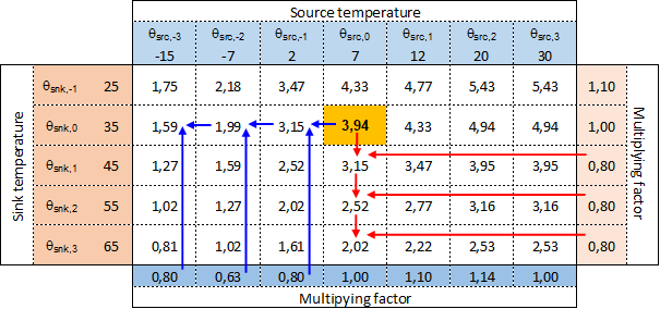
Figure 1. Sample performance map for an AW heat pump (full load COP).

If data from EN 14511 (or other typology specific standard) is known, the whole table can be filled in with the declared values. Examples are given in annex D of the draft review of the standard.

The principle is the same for all typologies of heat pumps. The reference temperatures only depend on the source and sink type. Heat pumps may also operate in summer, for domestic hot water service or if reheat is needed for dehumidification. In this case, the array of air source temperatures shall include values up to about 30°C. Extrapolation from 12°C is very likely to be inaccurate.

What is full load?

One potential issue is the definition of “full load”.

Obviously, for on-off heat pumps (or staged units with several on-off compressors) there is no doubt, there is only one possible operating condition at “full load”.

Modulating heat pump use a variable speed drive of the compressor, typically an inverter. In that case, the on-board software may intentionally limit the maximum compressor speed depending on the outdoor temperature. This makes sense because it is unlikely that you need the full power for heating at 15°C outdoor temperature, except if you also have to produce domestic hot water or if you need to recover after an indoor temperature set-back. This also avoids to operate in a condition where the power output is potentially very high and this requires oversized exchangers (evaporator and condenser) otherwise the COP drops because of their poor approach [1] at high power (see also next clause).

An example of such performance map with intentional heat output limitation is given in Figure 2, where the output power is electronically limited above −5°C. You may also note that data for domestic hot water operation are provided as well (12 to 30°C air temperature, 45 to 55 leaving water temperature).

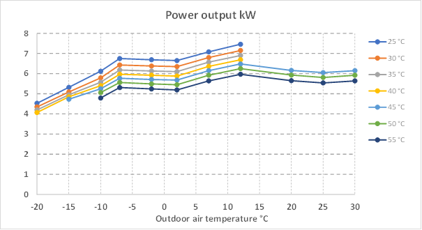
Figure 2. Sample performance map for an AW heat pump (full load power, electronically limited).

In this case, it should be taken into account that data above −5°C are not full load but already part load when performing the correction for part load operation. A possible solution is to report the compressor speed for each declared maximum power performance data. It is known and it would make it easy to avoid an incorrect estimation of part load correction.

How to correct for part load

There are several effects that may contribute to the change of COP at part load:

·         the decrease of the approach of evaporator and condenser, that results in lower temperature ad pressure difference between condenser and evaporator;

·         the change in heated fluid temperature difference (e.g. heated indoor air flowing through the condenser) when inlet temperature of heated fluid is used as a reference;

·         auxiliaries (such as evaporator fan or circulation pumps for an absorption heat pump) may run at constant or variable speed. At constant speed this allows a reduction of the approach due to less power to transfer but the relative effect of auxiliaries on COP increases.

An example of the effect of part load on operating conditions is given in figures 3 and 4 that show the temperatures in the refrigeration cycle of an air to water heat pump at full load and part load with the same source and sink temperature.

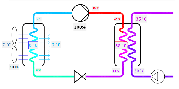
Figure 3. Example of full load operating conditions for an air to water heat pump.

Figure 4. Example of part load operating conditions for the same air to water heat pump.

The temperature difference between condenser and evaporator changes from 38°C (38–0) to 33°C (37–4). The contributing factors are:

·         a reduction of the outdoor air temperature drop on the evaporator (−3°C)

·         a reduction of the approach in the evaporator (−1°C)

·         a reduction of the approach in the condenser (-1°C)

This is likely to result in an increase of COP of 15%, if the compressor operates with the same II principle efficiency. Knowing the initial approaches and temperature differences on evaporator and condenser, it is an easy and reasonably accurate way to estimate the increase of the compressor efficiency at part load. However, you have to take into account also that the evaporator fan is running at constant speed, so this will affect more the COP at part load and partly compensate the increase in compressor COP.

A manufacturer may decide to reduce the evaporator fan speed at part load. In doing so, the auxiliary energy will be reduced but the reduction of the evaporator approach will be lost. This option could be triggered also by the intention to reduce noise of the outdoor unit.

In this draft review of the standard, several methods are proposed for the correction of COP at part load, which were already presented in the previous article:

·         default correction factors as a function of part load;

o   given as a series of tabulated values depending on the heat pump typology (for absorption heat pumps);

o   given as parameters for a standardised curve (optimum load factor, maximum increase of COP, etc) as specified in a DIN method for air to water heat pumps;

o   as a function of the parameters Cd (EN 14825 method), for ON-OFF operation

·         assuming a share of auxiliary power at full load and some increase of net compressor efficiency at an optimum part load (the method in the current version of the standard)

Which method to use depending on the heat pump typology and the required parameters are specified in tables B.11 through B.14 and B.42 in annex B to the draft EN 15316-4-2.

Specific features of path B

The principle

The intent of the so called “path B” is to leverage test data measured according to EN 14825.

The testing conditions considered by EN 14825 for air to air and air to water heat pumps are:

·         4 points at outdoor temperature of −7, +2, +7 and +12°C, identified by the letters A, B, C and D;

·         the “bivalent temperature”, labelled “BIV” (or “F”), at which it is assumed that the test load (called “building load”) matches the heat pump maximum output (i.e. CR is 100%, see previous article on heat pumps);

·         the minimum operating temperature of the heat pump, labelled “TOL” (or “E”) for temperature operation limit;

·         point “G” is an optional test point at −15°C, which is required only if SCOP for cold climate is declared.

The difficulty is that all three operating parameters (source and sink temperature, power output) are changing in each test point, according to the following rules.

·         Source temperature (external air temperature) TX is defined for points A, B, C, D (TA, TB, TC and TD) and optional point G (TG).

·         The sink temperature is 20°C for air-to-air heat pumps. It is a linear function of the external temperature for air-to-water heat pumps and values are shown in table 1 for medium temperature application.

·         The testing power PX is a linear function of external air temperature and the results are shown in Table 1. For the average climate, the design power PDES occurs at TDES= −10°C and PX=0 at 16°C.
However, if the heat pump operates ON-OFF in point D (and possibly C), then the COP is measured only in the ON condition and a degradation factor is used to correct the measured COP value.

The testing power is called “building load” because the heat demand decreasing linearly with outdoor temperature simulates the behaviour of a building. Actually, there is no building: this assumption is coupled with a bin distribution to generate a weighting factor of the measured COPs in the four test points A to D, to obtain the SCOP.

Given size of the heat pump, the testing power can be adjusted by the manufacturer. TBIV can be selected freely in the interval from TA to TDES. Two common choices are the following.

·         TBIV=TDES. This means that the heat pump can provide the whole fictive load in all test points and up to TDES = −10°C. No back-up energy is taken into account in the calculation of SCOP.

·         TBIV=TA. This means that the heat pump can provide the fictive load only until TBIV=TA= −7°C
The consequence is that in the determination of the SCOP, some back-up electric energy is included in the calculation, which reduces the COP at point A. This is possibly compensated by a reduced penalty at point D, where the heat pump may operate ON-OFF due to the minimum load.

The resulting test conditions combination is shown in Table 1 for the average climate and medium temperature application and for a heat pump that has an actual power output of 10 kW at −7°C, depending on the choice for TBIV.

Table 1. The resulting test conditions combination for the average climate and medium temperature application and for a heat pump that has an actual power output of 10 kW at −7°C, depending on the choice for TBIV.

It is obviously not easy to extract the influence of a single parameter from this data-set.

To overcome this difficulty, this calculation path assumes that the II principle efficiency [2] of the compressor be a function only of the required output power. This correlation is extracted once for all from the test data according to EN 14825. So, the procedure is:

·         calculate II principle efficiency dependency on the required output power;

·         calculate II principle efficiency for the required power output;

·         calculate COP based on source and sink temperature and II principle efficiency.

Figures 5 and 6 show the temperatures in an air to air heat pump at full load.

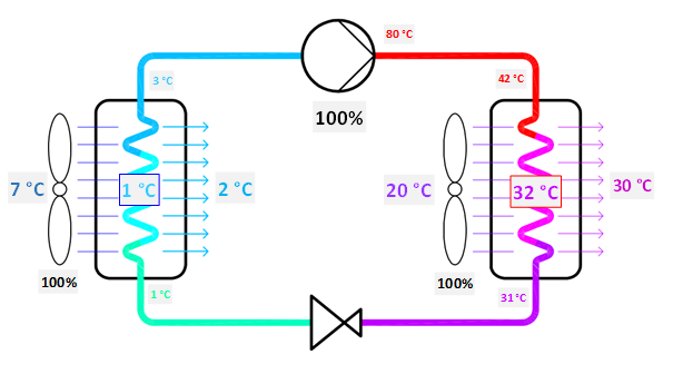
Figure 5. Example of full load operating conditions for an air-to-air heat pump.

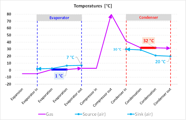
Figure 6. Example of full load temperature diagram along an air-to-air heat pump compression cycle.

The first part of the calculation method in path B aims at determining the evaporation and condensation temperature, given the source and sink temperatures and the power output in the available points. In the example shown in figures 5 and 6, the starting point are the temperatures of external air and indoor air, 7°C and 20°C respectively.

The first assumption is that the temperature difference between respectively:

·         the outdoor air (source) temperature (7°C) and the evaporation temperature (1°C)

·         the condensation temperature (32°C) and the indoor air (sink) temperature (20°C)

are proportional to the output power. This is the calculation performed in tables E.3 and E.5 of annex E to EN 15316-4-2.

It has to be noted that these differences are made of two components:

·         the approach of the condenser and the evaporator, which is likely to be proportional to power;

·         the temperature difference of the air flowing through the evaporator and through the condenser, which is proportional to the power if the air flow rate is constant.

As an example, looking at Figure 5, flowing through the condenser, indoor air temperature increases from 20 to 30°C at full load. The leaving air temperature will be 25°C at 50% load only if the indoor unit fan will be still running at full speed.

Once the evaporation and condensation temperature are known in the available test points, then the II principle efficiency is calculated for each available point and associated to the output power in that point.

The result is a function like the one in Figure 7.

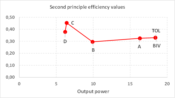
Figure 7. Example of resulting function: II principle efficiency as a function of output power.

At point D, the heat pump is often operating ON-OFF. That’s why points C and D are quite near in this example: test data in point D do not refer to the actual operating condition but only to the ON condition at minimum modulation. Then the measured COP value is corrected for intermittency using the Cd factor method.

The next step is calculating the evaporation and condensation temperature in the actual operating conditions in the calculation interval and the corresponding ideal COP using the Carnot equation.

Finally, you obtain the calculated COP at actual operating conditions by applying to the ideal COP the interpolated II principle efficiency at actual power output resulting from the function shown in Figure 7. If the actual output power is lower than that at point D (≈6 kW), then the actual COP at point D is further corrected for intermittency using the Cd factor method.

Again, it is assumed that the source and sink fluids flow rates in the evaporator and condenser stay constant. This means that the part load operating conditions corresponding to Figure 5 (full load operating conditions) should be as shown in Figure 8.

Figure 8. 50% load operating condition, coherent with path B assumptions and Figure 5 full load conditions.

The decrease in condensation temperature at part load (32°C to 26°C) is obtained if the air flow rate through the condenser stays constant. That’s one of the reasons for the COP peak at part load. If the condenser fan (indoor unit) modulates, then the operating conditions might be as shown in Figure 9.

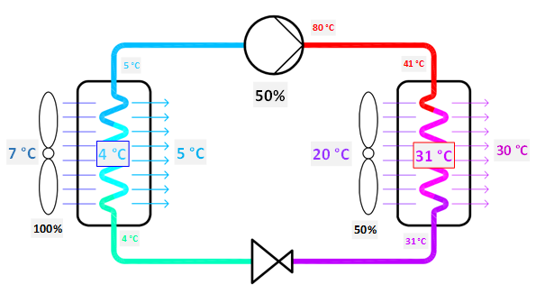
Figure 9. 50% load operating condition, if condenser fan modulates.

That means that “quiet operation” requires some trade-off between comfort and efficiency and the control strategy of the fan should be somehow taken into account. This is generally true, it is not a specific issue of path B.

Once evaporation and condensation temperatures are known in actual operating conditions, then the COP in the actual operating conditions is calculated according to the II principle efficiency at the actual output power.

Limitations of the current path B method

The current version of the path B method has some limitations in the possible use.

One limitation issues from the data-set provided by EN 14825: data on the maximum output power is available only for on-off heat pumps. For modulating heat pumps, it is assumed that the maximum power is that at the bivalent temperature. The increase in available power with higher source temperature is not described. This makes it difficult to handle situations with multiple generators, where one has to determine the contribution of each one based on their capacity.

Another limitation (also because of EN 14825 data-set) is the lack of information on the behaviour when producing domestic hot water and when operating in summer. A broad extrapolation would be required.

One or several path B

In the text of EN 15316-4-2 and in the accompanying spreadsheet, you will find separate clauses and separate calculation procedures for air to air and air to water heat pumps. The concept of the procedure is the same but the information available (input data list), the exceptions and particular cases have differences that make it simpler to have separate procedures.

The tables

In the examples in annex E (and in the current accompanying spreadsheet), calculation path B is demonstrated using tables. This is to better explain the procedure. In the revision following public enquiry the tables should disappear from the standard and the spreadsheet and shall be replaced by the required equations.

The entire calculation of the second principle efficiency as a function of the required output power (i.e. everything required to establish the graph in Figure 7) should be moved to a separate section to be applied only once for all when the product data of the heat pump is defined. There is no need to perform it at each calculation interval.

Further improvements

Transient deficit

A possible supplementary feature for the hourly method, is to allow a transient delay in the heat pump output. When there is a request for domestic hot water in one hour, it has priority over heating and it takes significant time to restore the set-point conditions into the storage. During peak heating request, the remaining time available in the hour can be too short to satisfy the heating demand, even at full load. Computationally there would be a part of the heating demand which is not satisfied. Actually, if the heat pump is correctly sized, this is just a transient deficit that will be recovered in the following hours. Due to the building time constant, the effect on comfort (temperature drop) is not perceivable. If the heat pump is undersized, the heat output deficit will not be recovered, it will increase hour by hour and day by day.

This feature can be easily introduced by:

·         saving as a calculation output the total heat deficit at the end of the current hour;

·         summing that total heat deficit to the heating needs at the beginning of the next hour.

If the total deficit is continuously increasing for several hours, this means that the heat pump is undersized.

If the total deficit has a sudden rise when domestic hot water service is requested and then decays in the next few hours, then this should be accepted.

With this feature, no advantage is given because needs are not reduced by a diminished internal temperature, which would be the case if the information about the actual reduced available power were passed to the heating needs module EN ISO 52016-1. In total, the heat pump will produce the whole heating needs but this will happen partly in the next hours with a higher load factor, just like things happen in reality. An example of such behaviour is shown in Figure 10.

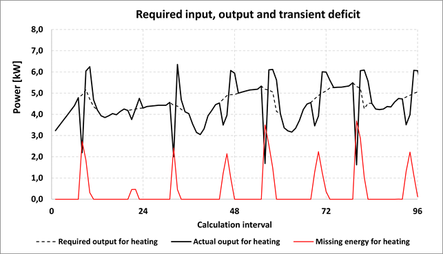
Figure 10. Example of transient heating power deficit.

Peaks of missing energy for heating are due to the heat request for the domestic hot water preparation (thermostat asking to restore the temperature in the domestic hot water storage).

A possible criterion is that the transient deficit can be considered acceptable if:

·         there are no more than 3 (or any other number) consecutive hours of increasing total heat deficit;

·         the deficit is again zero in a maximum of 6 (or any other number) hours.

If these criteria are not met, then a warning should be issued and the output power deficit handled as a true one.

This is also useful as a filter to sudden surges of heating needs power generated by EN ISO 52016-1, that are due to the assumption of perfect temperature control. A step in gains is automatically transformed into an instantaneous step in heating (or cooling) needs whilst in reality it takes some time and some indoor temperature drift for the system to react.

Domestic hot water only

The case of domestic hot water only should be further refined, taken into account into the priority criterion and a better connection should be sought with the specific product standard.

A clarification about the meaning of the “thermostat-off”, “stand-by” and “crankcase heating” auxiliary power defined in EN 14825 is needed. As an example, it’s difficult to understand what can be the difference between “thermostat-off” and “stand-by”.

Publication

The new draft will be sent by CEN central secretariat to the national standardisation bodies for the public enquiry in the coming months.

The accompanying demonstration spreadsheet will be published on EPB-Center website, together with a short video explaining the calculation method and the features of the spreadsheet.

If you read this article, you should be ready for the impact.

Have fun in commenting the new draft for EN 15316-4-2.

Literature

Heat pumps: lost in standards…, Laurent Socal, REHVA Journal 2020-04 (https://www.rehva.eu/rehva-journal/chapter/heat-pumps-lost-in-standards)

Standards

prEN 15316-4-2: 2021 Energy performance of buildings — Method for calculation of system energy requirements and system efficiencies – Part 4-2: Space heating generation systems, heat pump systems, Module M3-8-2, M8-8-2 (publication for enquiry expected late autumn 2021).

EN 15316-4-2:2017 Energy performance of buildings - Method for calculation of system energy requirements and system efficiencies – Part 4-2: Space heating generation systems, heat pump systems, Module M3-8-2, M8-8-2.

EN 15316-1: 2017 Energy performance of buildings - Method for calculation of system energy requirements and system efficiencies – Part 1: General and Energy performance expression, Module M3-1, M3-4, M3- 9, M8-1, M8-4.

EN 14511:2018 Air conditioners, liquid chilling packages and heat pumps for space heating and cooling and process chillers, with electrically driven compressors – Part 1: Terms and definitions; Part 2: Test conditions; Part 3: Test methods; Part 4: Requirements.

EN 14825:2018 Air conditioners, liquid chilling packages and heat pumps, with electrically driven compressors, for space heating and cooling, commercial and process cooling - Testing and rating at part load conditions and calculation of seasonal performance. (currently under revision, the prEN was published in 2020).

References